

An Array of Cells
In order to produce a list of data, the spreadsheets provide a feature called arrays or more relevantly an array of cells that could be filled in to compile a list.
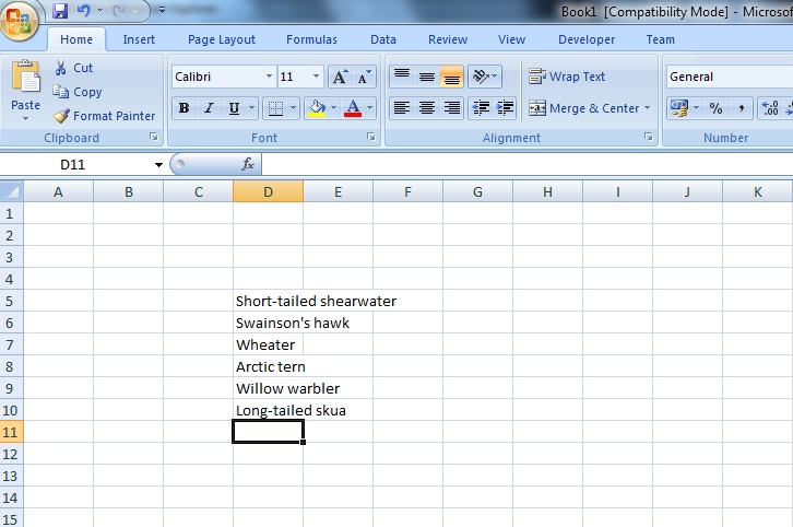
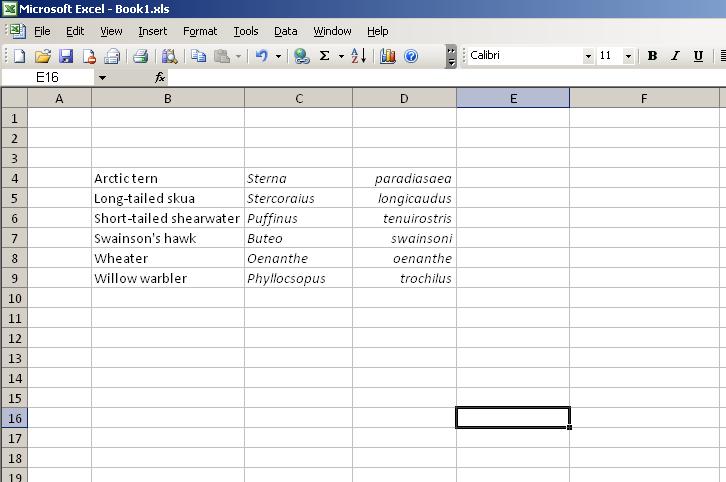
The lines which are displayed within the image above are regarded as an important feature to the overall layout of the excel software or more specifically the GUI (Graphical User Interface), the reason why these are implmented into the interface is that they can aid the user to select which location would be most appropriate for them to input the neccessary and desired data.
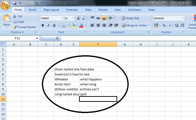
It is apparant that some of the text that is displayed within the line areas do not completely fit into the location and seem to expand and pass into the slot located beside the slot that the text is written in. These slots are also known as cells and are widened automatically and do not trim the text or become hidden regardless of the original size of the cells, the text is only trimmed when the cells next to the lengthened text data are also occupied with text as well such as the example displayed below.
Sorting the Data
A frequent and standard technique that is used on any type of list, in particular when it becomes long, is to organize the data in some sort of order, most commonly in alphabetical order, this is known as sorting. The facilities available within the excel software allows this sorting ability to be very simple and can be carried out with ease.
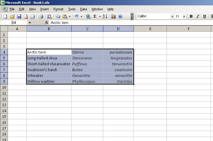
In order for the sorting to be successful there must be a selection towards what details or set of data is required to be sorted, this is done by highlighting the entire list by clicking on the first cell of the set of data with the cursor then holding onto the click and dragging through the list unto the final cell within that set of data.
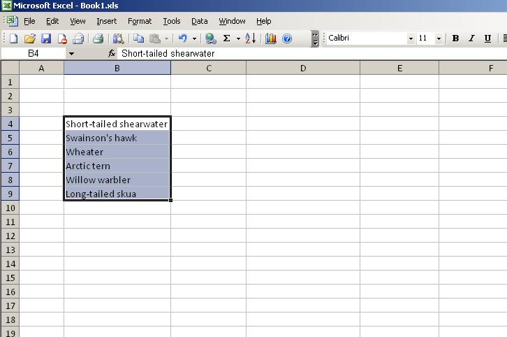
As can be seen within the image, all of the data that has been selected is contrasted in a blue colour around the cells with the exception of the white cell, which also belongs to the highlighted data set but the reason due to this cell being of a distinct colour to the rest is that it is the initial cell that is selected. After all of this is complete then the sort function needs to be searched for which is stored within the menu called items, it provides the option to either sort the information into descending order or ascending order. If ascending order is chosen for example, the following table within the screenshot below is produced.
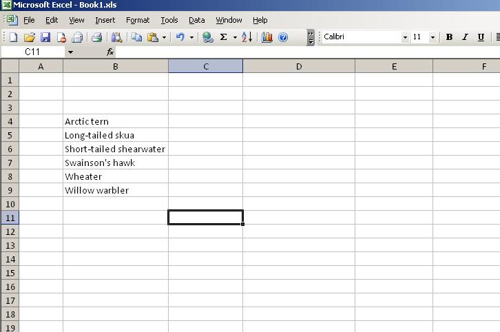
It can be clarified that the order of the data has been changed and this is also in accordance to the first letter of each piece of text data as they all enlist in alphabetical order.
This is also related with the spreadsheet view as the cell data is "atomic" or "monolithic" from the computer's perspective which means that the computer itself does not take into account any of the data's independent parts.
Adding More Data To The List
Based upon the example that has been used of the table of data, it is possible to add new categories of data which relate to what is already available in the table, these could be placed within the columns directly beside the list currently within the table, these two categories could consist of genus and also the species of the birds.
Since genus and species comprise of terms which are scientific, they are generally displayed in italic form, this can be applied upon the new data sets with the formatting features which belong to the excel spreadsheet software, the same type that can be found in word processors which can alter wording to italics, change boldness, adjust the font styles, font sizes, the justification, the colour etc..
Within the Excel spreadsheet software package, the formatting features are stored within the FORMAT menu, within this instance the scientific names will be converted to italics and the genus names will be right justified so it is paired with the species name.
If now the whole table of data is to be sorted in relation to the other categories that have just been inputted then the first step is to highlight the entire data set such as the example below.
We then enter the sorting feature within the spreadsheet software, The design of the spreadsheet program of excel includes within it references for each column and row which can be used more closely to define each and every cell of the spreadsheet, if we wish to reorder the whole entire table based upon a particular column i.e. column C, or by a particular row i.e. row 4 or by a single cell (which is determined by the combination of the column reference as well as the row reference so if this cell is in column B and row 4 then the cell name is B4), then this can be processed into the sorting window which is presented below.

The table of data has been sorted by the set of information that is allocated within column C (the information for the Genuses), the following result is produced when the directional arrow is clicked.

Also on a side note a particular group of cells can be selected by specifying the very first cell of the group as the first cell name i.e. B2 then this is followed by a : and the final cell name after the colon is the very final cell within the selected group such as D7 for example so this results as B2:D7, this type of term is known as a "Cell Range", the cell range B4:D9 is highlighted in the example above.
Demo Of Creating A Spreadsheet And Sorting Data
Below is a video clip tutorial showcasing how to construct a spreadsheet, edit the text data within the cells and also sort the data into order.